Inferential statistics
https://www.khanacademy.org/math/probability/statistics-inferential
Confidence interval 1
Estimating the probability that the true population mean lies within a range around a sample mean.

Confidence interval example
Confidence Interval Example

Small sample size confidence intervals
Constructing small sample size confidence

Constructing small sample size confidence
Student's t-distribution
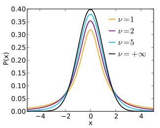
Probability density function[edit]
Student's t-distribution has the probability density function given by

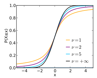
CDF
![\begin{matrix}
\frac{1}{2} + x \Gamma \left( \frac{\nu+1}{2} \right) \times\\[0.5em]
\frac{\,_2F_1 \left ( \frac{1}{2},\frac{\nu+1}{2};\frac{3}{2};
-\frac{x^2}{\nu} \right)}
{\sqrt{\pi\nu}\,\Gamma \left(\frac{\nu}{2}\right)}
\end{matrix}](http://upload.wikimedia.org/math/a/b/7/ab74f89cdde5da4507cddc3607c9cf1d.png)
One Sided 75% 80% 85% 90% 95% 97.5% 99% 99.5% 99.75% 99.9% 99.95% Two Sided 50% 60% 70% 80% 90% 95% 98% 99% 99.5% 99.8% 99.9% 1 1.000 1.376 1.963 3.078 6.314 12.71 31.82 63.66 127.3 318.3 636.6 2 0.816 1.061 1.386 1.886 2.920 4.303 6.965 9.925 14.09 22.33 31.60 3 0.765 0.978 1.250 1.638 2.353 3.182 4.541 5.841 7.453 10.21 12.92 4 0.741 0.941 1.190 1.533 2.132 2.776 3.747 4.604 5.598 7.173 8.610 5 0.727 0.920 1.156 1.476 2.015 2.571 3.365 4.032 4.773 5.893 6.869 6 0.718 0.906 1.134 1.440 1.943 2.447 3.143 3.707 4.317 5.208 5.959 7 0.711 0.896 1.119 1.415 1.895 2.365 2.998 3.499 4.029 4.785 5.408 8 0.706 0.889 1.108 1.397 1.860 2.306 2.896 3.355 3.833 4.501 5.041 9 0.703 0.883 1.100 1.383 1.833 2.262 2.821 3.250 3.690 4.297 4.781 10 0.700 0.879 1.093 1.372 1.812 2.228 2.764 3.169 3.581 4.144 4.587 11 0.697 0.876 1.088 1.363 1.796 2.201 2.718 3.106 3.497 4.025 4.437 12 0.695 0.873 1.083 1.356 1.782 2.179 2.681 3.055 3.428 3.930 4.318 13 0.694 0.870 1.079 1.350 1.771 2.160 2.650 3.012 3.372 3.852 4.221 14 0.692 0.868 1.076 1.345 1.761 2.145 2.624 2.977 3.326 3.787 4.140 15 0.691 0.866 1.074 1.341 1.753 2.131 2.602 2.947 3.286 3.733 4.073 16 0.690 0.865 1.071 1.337 1.746 2.120 2.583 2.921 3.252 3.686 4.015 17 0.689 0.863 1.069 1.333 1.740 2.110 2.567 2.898 3.222 3.646 3.965 18 0.688 0.862 1.067 1.330 1.734 2.101 2.552 2.878 3.197 3.610 3.922 19 0.688 0.861 1.066 1.328 1.729 2.093 2.539 2.861 3.174 3.579 3.883 20 0.687 0.860 1.064 1.325 1.725 2.086 2.528 2.845 3.153 3.552 3.850 21 0.686 0.859 1.063 1.323 1.721 2.080 2.518 2.831 3.135 3.527 3.819 22 0.686 0.858 1.061 1.321 1.717 2.074 2.508 2.819 3.119 3.505 3.792 23 0.685 0.858 1.060 1.319 1.714 2.069 2.500 2.807 3.104 3.485 3.767 24 0.685 0.857 1.059 1.318 1.711 2.064 2.492 2.797 3.091 3.467 3.745 25 0.684 0.856 1.058 1.316 1.708 2.060 2.485 2.787 3.078 3.450 3.725 26 0.684 0.856 1.058 1.315 1.706 2.056 2.479 2.779 3.067 3.435 3.707 27 0.684 0.855 1.057 1.314 1.703 2.052 2.473 2.771 3.057 3.421 3.690 28 0.683 0.855 1.056 1.313 1.701 2.048 2.467 2.763 3.047 3.408 3.674 29 0.683 0.854 1.055 1.311 1.699 2.045 2.462 2.756 3.038 3.396 3.659 30 0.683 0.854 1.055 1.310 1.697 2.042 2.457 2.750 3.030 3.385 3.646 40 0.681 0.851 1.050 1.303 1.684 2.021 2.423 2.704 2.971 3.307 3.551 50 0.679 0.849 1.047 1.299 1.676 2.009 2.403 2.678 2.937 3.261 3.496 60 0.679 0.848 1.045 1.296 1.671 2.000 2.390 2.660 2.915 3.232 3.460 80 0.678 0.846 1.043 1.292 1.664 1.990 2.374 2.639 2.887 3.195 3.416 100 0.677 0.845 1.042 1.290 1.660 1.984 2.364 2.626 2.871 3.174 3.390 120 0.677 0.845 1.041 1.289 1.658 1.980 2.358 2.617 2.860 3.160 3.373 
0.674 0.842 1.036 1.282 1.645 1.960 2.326 2.576 2.807 3.090 3.291
 is the number of
  is the
 CDF
| One Sided | 75% | 80% | 85% | 90% | 95% | 97.5% | 99% | 99.5% | 99.75% | 99.9% | 99.95% |
|---|---|---|---|---|---|---|---|---|---|---|---|
| Two Sided | 50% | 60% | 70% | 80% | 90% | 95% | 98% | 99% | 99.5% | 99.8% | 99.9% |
| 1 | 1.000 | 1.376 | 1.963 | 3.078 | 6.314 | 12.71 | 31.82 | 63.66 | 127.3 | 318.3 | 636.6 |
| 2 | 0.816 | 1.061 | 1.386 | 1.886 | 2.920 | 4.303 | 6.965 | 9.925 | 14.09 | 22.33 | 31.60 |
| 3 | 0.765 | 0.978 | 1.250 | 1.638 | 2.353 | 3.182 | 4.541 | 5.841 | 7.453 | 10.21 | 12.92 |
| 4 | 0.741 | 0.941 | 1.190 | 1.533 | 2.132 | 2.776 | 3.747 | 4.604 | 5.598 | 7.173 | 8.610 |
| 5 | 0.727 | 0.920 | 1.156 | 1.476 | 2.015 | 2.571 | 3.365 | 4.032 | 4.773 | 5.893 | 6.869 |
| 6 | 0.718 | 0.906 | 1.134 | 1.440 | 1.943 | 2.447 | 3.143 | 3.707 | 4.317 | 5.208 | 5.959 |
| 7 | 0.711 | 0.896 | 1.119 | 1.415 | 1.895 | 2.365 | 2.998 | 3.499 | 4.029 | 4.785 | 5.408 |
| 8 | 0.706 | 0.889 | 1.108 | 1.397 | 1.860 | 2.306 | 2.896 | 3.355 | 3.833 | 4.501 | 5.041 |
| 9 | 0.703 | 0.883 | 1.100 | 1.383 | 1.833 | 2.262 | 2.821 | 3.250 | 3.690 | 4.297 | 4.781 |
| 10 | 0.700 | 0.879 | 1.093 | 1.372 | 1.812 | 2.228 | 2.764 | 3.169 | 3.581 | 4.144 | 4.587 |
| 11 | 0.697 | 0.876 | 1.088 | 1.363 | 1.796 | 2.201 | 2.718 | 3.106 | 3.497 | 4.025 | 4.437 |
| 12 | 0.695 | 0.873 | 1.083 | 1.356 | 1.782 | 2.179 | 2.681 | 3.055 | 3.428 | 3.930 | 4.318 |
| 13 | 0.694 | 0.870 | 1.079 | 1.350 | 1.771 | 2.160 | 2.650 | 3.012 | 3.372 | 3.852 | 4.221 |
| 14 | 0.692 | 0.868 | 1.076 | 1.345 | 1.761 | 2.145 | 2.624 | 2.977 | 3.326 | 3.787 | 4.140 |
| 15 | 0.691 | 0.866 | 1.074 | 1.341 | 1.753 | 2.131 | 2.602 | 2.947 | 3.286 | 3.733 | 4.073 |
| 16 | 0.690 | 0.865 | 1.071 | 1.337 | 1.746 | 2.120 | 2.583 | 2.921 | 3.252 | 3.686 | 4.015 |
| 17 | 0.689 | 0.863 | 1.069 | 1.333 | 1.740 | 2.110 | 2.567 | 2.898 | 3.222 | 3.646 | 3.965 |
| 18 | 0.688 | 0.862 | 1.067 | 1.330 | 1.734 | 2.101 | 2.552 | 2.878 | 3.197 | 3.610 | 3.922 |
| 19 | 0.688 | 0.861 | 1.066 | 1.328 | 1.729 | 2.093 | 2.539 | 2.861 | 3.174 | 3.579 | 3.883 |
| 20 | 0.687 | 0.860 | 1.064 | 1.325 | 1.725 | 2.086 | 2.528 | 2.845 | 3.153 | 3.552 | 3.850 |
| 21 | 0.686 | 0.859 | 1.063 | 1.323 | 1.721 | 2.080 | 2.518 | 2.831 | 3.135 | 3.527 | 3.819 |
| 22 | 0.686 | 0.858 | 1.061 | 1.321 | 1.717 | 2.074 | 2.508 | 2.819 | 3.119 | 3.505 | 3.792 |
| 23 | 0.685 | 0.858 | 1.060 | 1.319 | 1.714 | 2.069 | 2.500 | 2.807 | 3.104 | 3.485 | 3.767 |
| 24 | 0.685 | 0.857 | 1.059 | 1.318 | 1.711 | 2.064 | 2.492 | 2.797 | 3.091 | 3.467 | 3.745 |
| 25 | 0.684 | 0.856 | 1.058 | 1.316 | 1.708 | 2.060 | 2.485 | 2.787 | 3.078 | 3.450 | 3.725 |
| 26 | 0.684 | 0.856 | 1.058 | 1.315 | 1.706 | 2.056 | 2.479 | 2.779 | 3.067 | 3.435 | 3.707 |
| 27 | 0.684 | 0.855 | 1.057 | 1.314 | 1.703 | 2.052 | 2.473 | 2.771 | 3.057 | 3.421 | 3.690 |
| 28 | 0.683 | 0.855 | 1.056 | 1.313 | 1.701 | 2.048 | 2.467 | 2.763 | 3.047 | 3.408 | 3.674 |
| 29 | 0.683 | 0.854 | 1.055 | 1.311 | 1.699 | 2.045 | 2.462 | 2.756 | 3.038 | 3.396 | 3.659 |
| 30 | 0.683 | 0.854 | 1.055 | 1.310 | 1.697 | 2.042 | 2.457 | 2.750 | 3.030 | 3.385 | 3.646 |
| 40 | 0.681 | 0.851 | 1.050 | 1.303 | 1.684 | 2.021 | 2.423 | 2.704 | 2.971 | 3.307 | 3.551 |
| 50 | 0.679 | 0.849 | 1.047 | 1.299 | 1.676 | 2.009 | 2.403 | 2.678 | 2.937 | 3.261 | 3.496 |
| 60 | 0.679 | 0.848 | 1.045 | 1.296 | 1.671 | 2.000 | 2.390 | 2.660 | 2.915 | 3.232 | 3.460 |
| 80 | 0.678 | 0.846 | 1.043 | 1.292 | 1.664 | 1.990 | 2.374 | 2.639 | 2.887 | 3.195 | 3.416 |
| 100 | 0.677 | 0.845 | 1.042 | 1.290 | 1.660 | 1.984 | 2.364 | 2.626 | 2.871 | 3.174 | 3.390 |
| 120 | 0.677 | 0.845 | 1.041 | 1.289 | 1.658 | 1.980 | 2.358 | 2.617 | 2.860 | 3.160 | 3.373 |
| 0.674 | 0.842 | 1.036 | 1.282 | 1.645 | 1.960 | 2.326 | 2.576 | 2.807 | 3.090 | 3.291 |
How the t-distribution arises
Sampling distribution
Let x1, ..., xn be the numbers observed in a sample
from a continuously distributed population with expected value μ.
The sample mean and sample variance are given by:

The resulting t-value is

Suppose X1, ..., Xn are independent realizations
of the normally-distributed, random variable X,
which has an expected value μ and variance σ2.
Let


==>
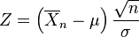
is normally distributed with mean 0 and variance 1,

has a chi-squared distribution with v=n−1 degrees of freedom

has a Student's t-distribution with v=n−1 degrees of freedom
| Parameters | ν = (n-1)> 0 degrees of freedom (real) |
|---|
| Mean | 0 for ν > 1, otherwise undefined |
|---|
| Variance |  for ν > 2, ∞ for 1 < ν ≤ 2, otherwiseundefined for ν > 2, ∞ for 1 < ν ≤ 2, otherwiseundefined |
|---|
 |
| CDF | where 2F1 is the hypergeometric function |
|---|
Density of the t-distribution (red) for 1, 5, and 30 degrees of freedom
compared to the standard normal distribution (blue).
Previous plots shown in green.


Normal Distribution for Z value:


T distribution for T value, with v= inf, v=10, v=1
blue: Normal, 95% ==> 1.96
red: T, v= 10, 95% ==> 2.28
green: T, v=1, 95% ==> 12.71
沒有留言:
張貼留言